Learn how to achieve precise detection of tiny objects (like small clips) on the RDK X5, without adding any inference latency, simply by improving the YOLOv5s loss function.
1. Model Introduction
※Reference Links
-
YOLOv5: https://github.com/ultralytics/yolov5/blob/v7.0/README.md
-
NWD Paper: https://arxiv.org/abs/2005.03572
Small object detection has always been a tough nut to crack. Targets like “small binder clips” occupy very few pixels in an image, and traditional IoU-based loss functions are extremely sensitive to positional deviations — two boxes may both have an IoU of zero, yet their actual spatial relationship to the ground truth can be wildly different.
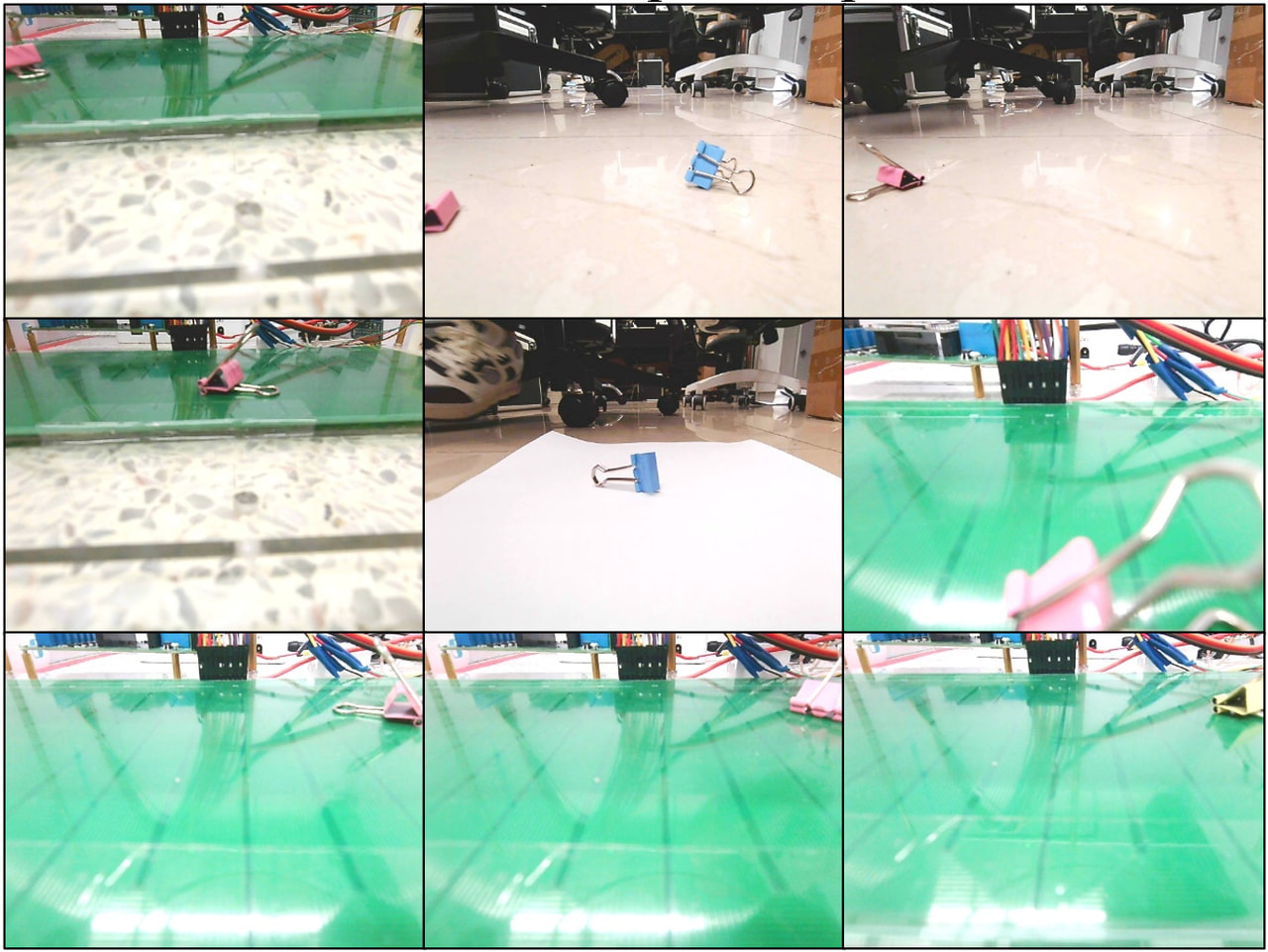
Core idea: NWD Loss. Normalized Wasserstein Distance (NWD) models each bounding box as a 2D Gaussian distribution and computes the Wasserstein distance between these distributions as the regression loss. Even when two boxes do not overlap at all, NWD still provides a meaningful distance metric and a smooth, effective gradient, avoiding the vanishing gradient problem. Previous work has shown that YOLOv5-NWD can improve accuracy by 7.2% and F1 score by 2.2% on a small-object corrosion detection task.
Our modification: We only replaced the original IoU loss with NWD loss in the utils/loss.py file of the YOLOv5s source code. The model architecture itself remains untouched — no extra detection heads, no attention modules. This means the forward pass during inference is completely unchanged; all accuracy gains come from better model parameters.
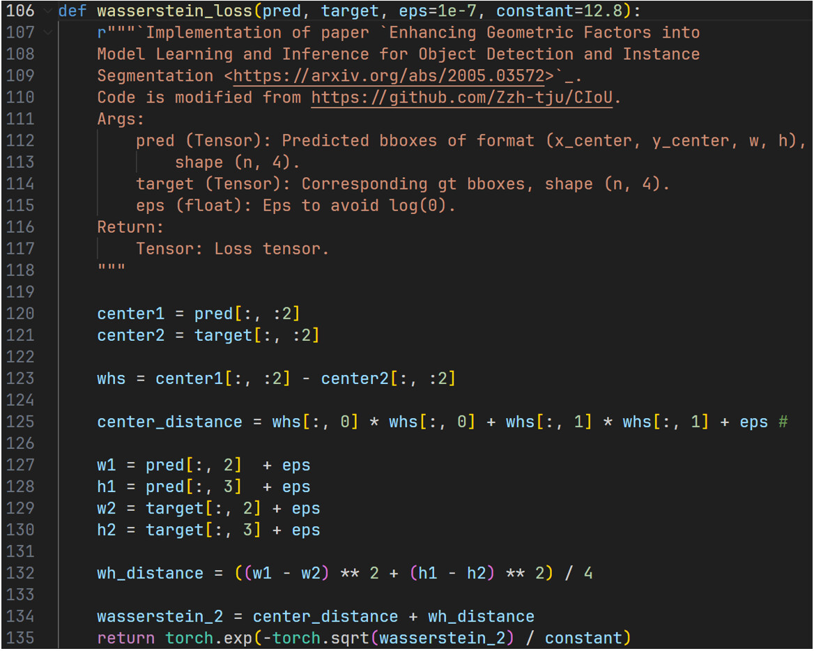
'''NWD Loss Function'''
def wasserstein_loss(pred, target, eps=1e-7, constant=12.8):
    r"""`Implementation of paper `Enhancing Geometric Factors into
    Model Learning and Inference for Object Detection and Instance
    Segmentation <https://arxiv.org/abs/2005.03572>`_.
    Code is modified from https://github.com/Zzh-tju/CIoU.
    Args:
        pred (Tensor): Predicted bboxes of format (x_center, y_center, w, h),
            shape (n, 4).
        target (Tensor): Corresponding gt bboxes, shape (n, 4).
        eps (float): Eps to avoid log(0).
    Return:
        Tensor: Loss tensor.
    """

    center1 = pred[:, :2]
    center2 = target[:, :2]

    whs = center1[:, :2] - center2[:, :2]

    center_distance = whs[:, 0] * whs[:, 0] + whs[:, 1] * whs[:, 1] + eps #

    w1 = pred[:, 2]  + eps
    h1 = pred[:, 3]  + eps
    w2 = target[:, 2] + eps
    h2 = target[:, 3] + eps

    wh_distance = ((w1 - w2) ** 2 + (h1 - h2) ** 2) / 4

    wasserstein_2 = center_distance + wh_distance
    return torch.exp(-torch.sqrt(wasserstein_2) / constant
# lbox += (1.0 - iou).mean()  # iou loss

# # Objectness
# iou = iou.detach().clamp(0).type(tobj.dtype)
'''For NWD loss function'''
nwd = wasserstein_loss(pbox, tbox[i]).squeeze()
iou_ratio = 0.5
lbox += (1 - iou_ratio) * (1.0 - nwd).mean() + iou_ratio * (1.0 - iou).mean()  # iou loss

# Objectness
iou = (iou.detach() * iou_ratio + nwd.detach() * (1 - iou_ratio)).clamp(0, 1).type(tobj.dtype)
'''For NWD loss function''
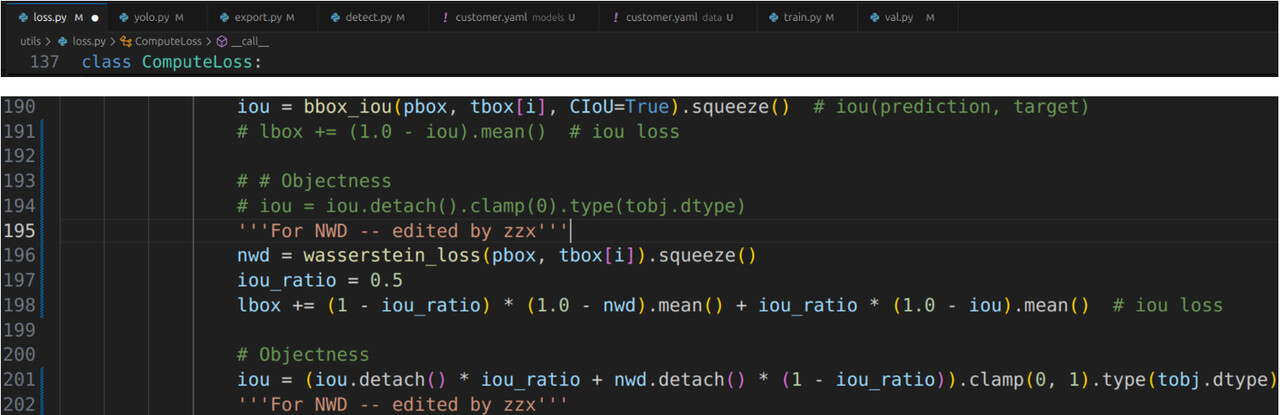
The final joint loss function is as follows, where iou_ratio ∈ [0,1] is a tunable parameter:

A comparison between the modified model and the original YOLOv5s is shown below.
| Comparison Item | Original YOLOv5s | NWD-YOLOv5s |
|---|---|---|
| Model Structure | Standard YOLOv5s | the same |
| Loss Function | IoU-based | Iou+NWD-based |
| Inference Path | — | the same |
| Parameter Count | — | the same |
The final training results are summarized in the following table.
| loss function | Prediction accuracy | Recall rate | mAP50 | mAP50-95 |
|---|---|---|---|---|
| IoU | 0.995 | 1 | 0.995 | 0.827 |
| IoU+NWD | 0.998 | 1 | 0.995 | 0.841 |

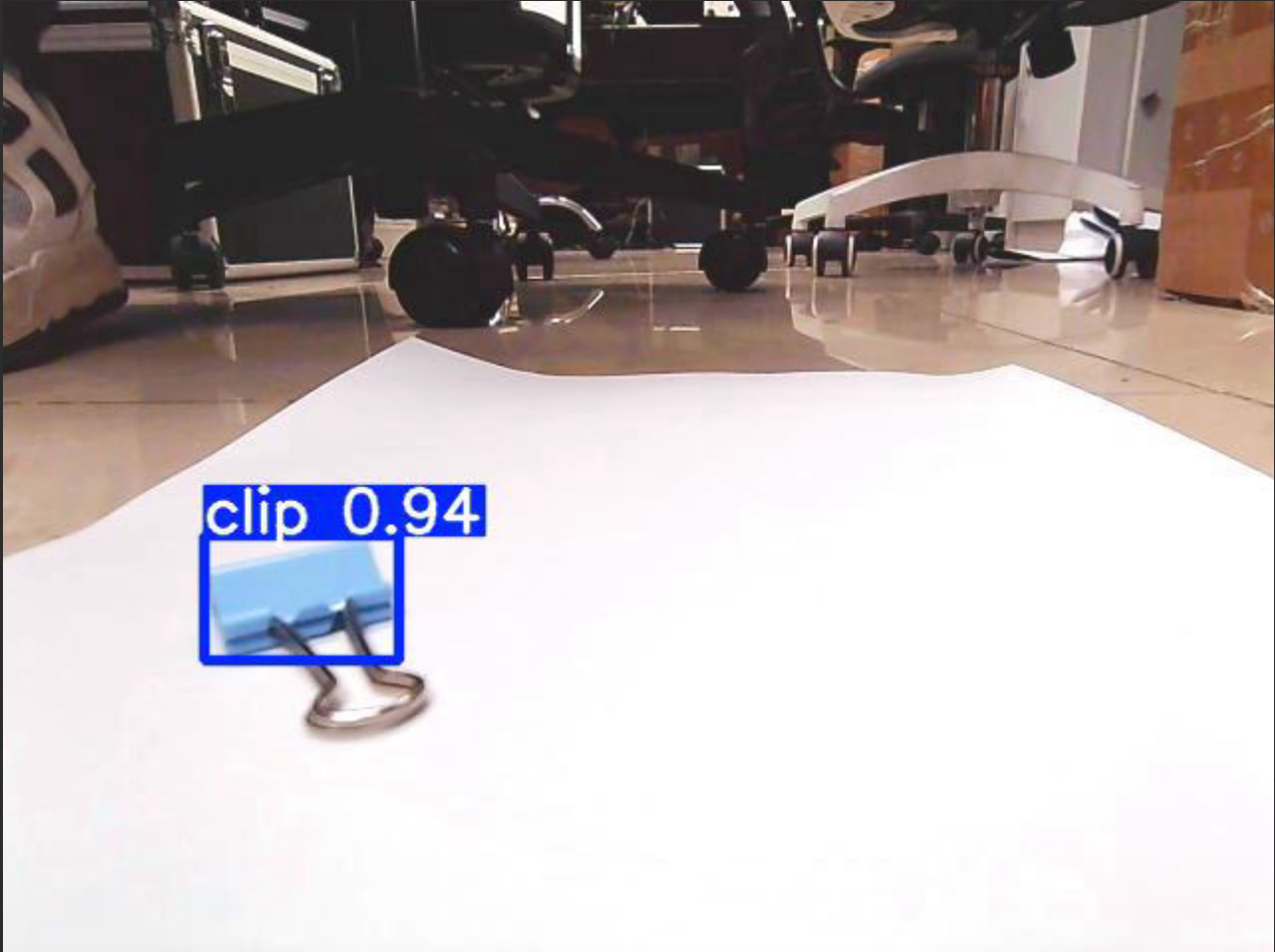
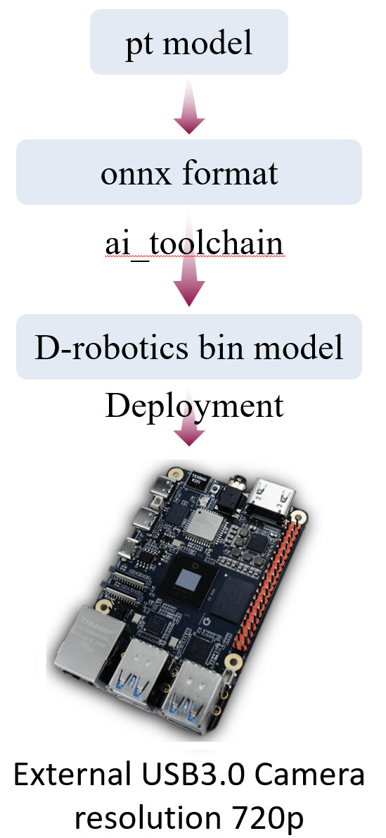
Next, we will convert the PyTorch model to ONNX format, then quantize it using the Horizon Algorithm Toolchain, and finally deploy the .bin quantized model on the RDK X5 to perform small-object detection on a USB camera video stream.
The Deployment pipeline is as follows.
2. ONNX Model
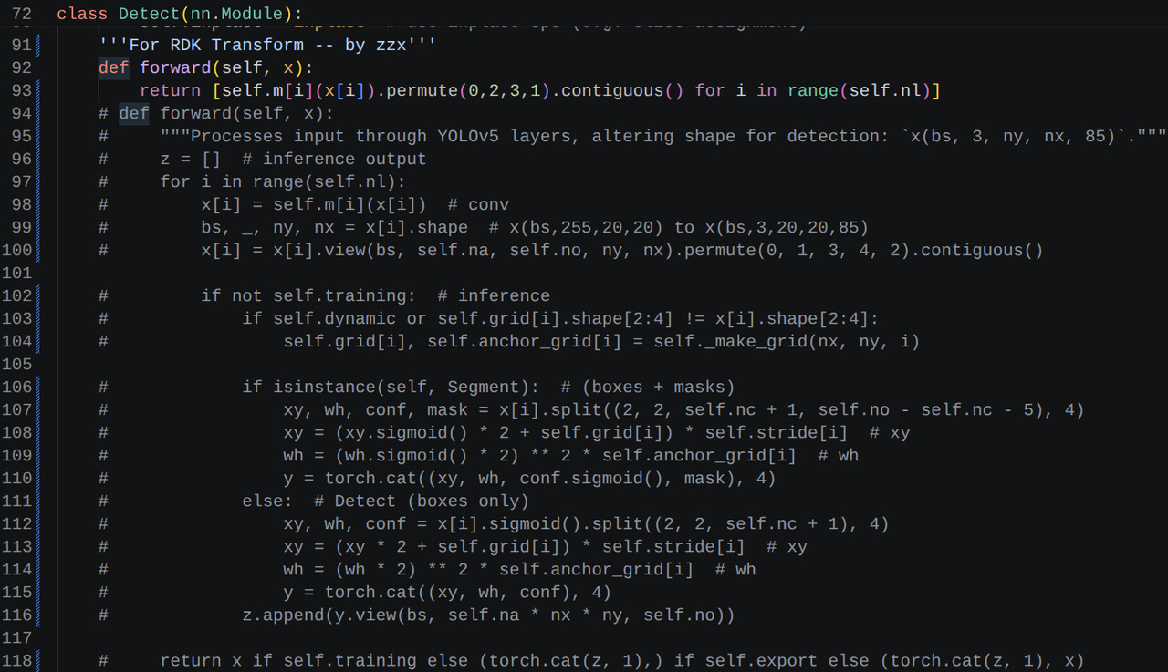
Before conversion, if you’re using the yolov5-v7.0 code, you need to modify the forward member function of the Detect class in model/yolo.py, as follows.
The goal is to have the function return directly to the original feature map of each detector head after convolution, and adjust the dimensional order. That is, the model is only responsible for “feature extraction,” in line with best practices for edge deployment.
    '''For RDK Output onnx'''
    def forward(self, x):
        return [self.m[i](x[i]).permute(0,2,3,1).contiguous() for i in range(self.nl)]
    # def forward(self, x):
    #     """Processes input through YOLOv5 layers, altering shape for detection: `x(bs, 3, ny, nx, 85)`."""
    #     z = []  # inference output
    #     for i in range(self.nl):
    #         x[i] = self.m[i](x[i])  # conv
    #         bs, _, ny, nx = x[i].shape  # x(bs,255,20,20) to x(bs,3,20,20,85)
    #         x[i] = x[i].view(bs, self.na, self.no, ny, nx).permute(0, 1, 3, 4, 2).contiguous()

    #         if not self.training:  # inference
    #             if self.dynamic or self.grid[i].shape[2:4] != x[i].shape[2:4]:
    #                 self.grid[i], self.anchor_grid[i] = self._make_grid(nx, ny, i)

    #             if isinstance(self, Segment):  # (boxes + masks)
    #                 xy, wh, conf, mask = x[i].split((2, 2, self.nc + 1, self.no - self.nc - 5), 4)
    #                 xy = (xy.sigmoid() * 2 + self.grid[i]) * self.stride[i]  # xy
    #                 wh = (wh.sigmoid() * 2) ** 2 * self.anchor_grid[i]  # wh
    #                 y = torch.cat((xy, wh, conf.sigmoid(), mask), 4)
    #             else:  # Detect (boxes only)
    #                 xy, wh, conf = x[i].sigmoid().split((2, 2, self.nc + 1), 4)
    #                 xy = (xy * 2 + self.grid[i]) * self.stride[i]  # xy
    #                 wh = (wh * 2) ** 2 * self.anchor_grid[i]  # wh
    #                 y = torch.cat((xy, wh, conf), 4)
    #             z.append(y.view(bs, self.na * nx * ny, self.no))

    #     return x if self.training else (torch.cat(z, 1),) if self.export else (torch.cat(z, 1), x
※Note: When you want to retrain .pt model, be sure to undo the changes to the forward function.
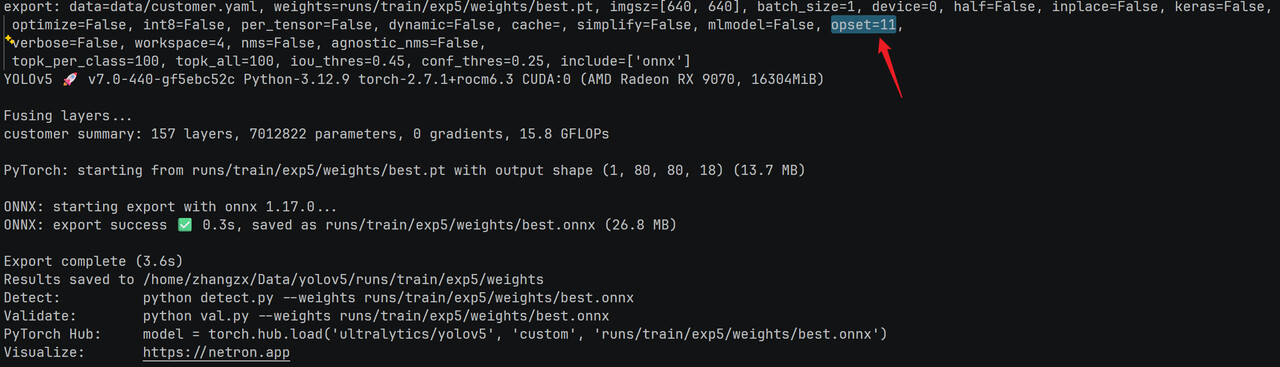
Then, export the PyTorch model to ONNX format, ensuring the opset version is set to 11 — a critical step for compatibility with the Horizon Algorithm Toolchain.
For RDK X5, only operators with opset version 11 and below are supported. See the development manual.
parser.add_argument("--opset", type=int, default=11, help="ONNX: opset version"
default=["onnx"] #on line 1540

The exported ONNX model is structurally identical to the standard YOLOv5s. It is recommended to run a sanity check with ONNXRuntime before proceeding to quantization to confirm there is no accuracy degradation.
3. Model Quantization
We will use the Horizon Algorithm Toolchain (OpenExplorer) to quantize the ONNX model into a .bin file that can run on the BPU.
-
Environment: Horizon’s official Docker image
openexplorer/ai_toolchain_ubuntu_20_x5_cpu:v1.2.8— no local dependency hassle. -
Preprocessing: Check ONNX operator compatibility with
hb_mapper; configure the YAML file to specify the calibration dataset path and output nodes. -
Quantization & Compilation example command:
hb_mapper makertbin --config path/to/your/config.yaml --model-type onnx
※Note: Since the NWD modification only affects loss calculation during training, the operators during inference are exactly the same as the original YOLOv5s. Therefore, there are zero additional compatibility issues during quantization.
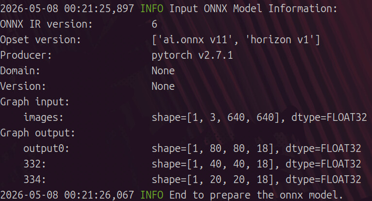
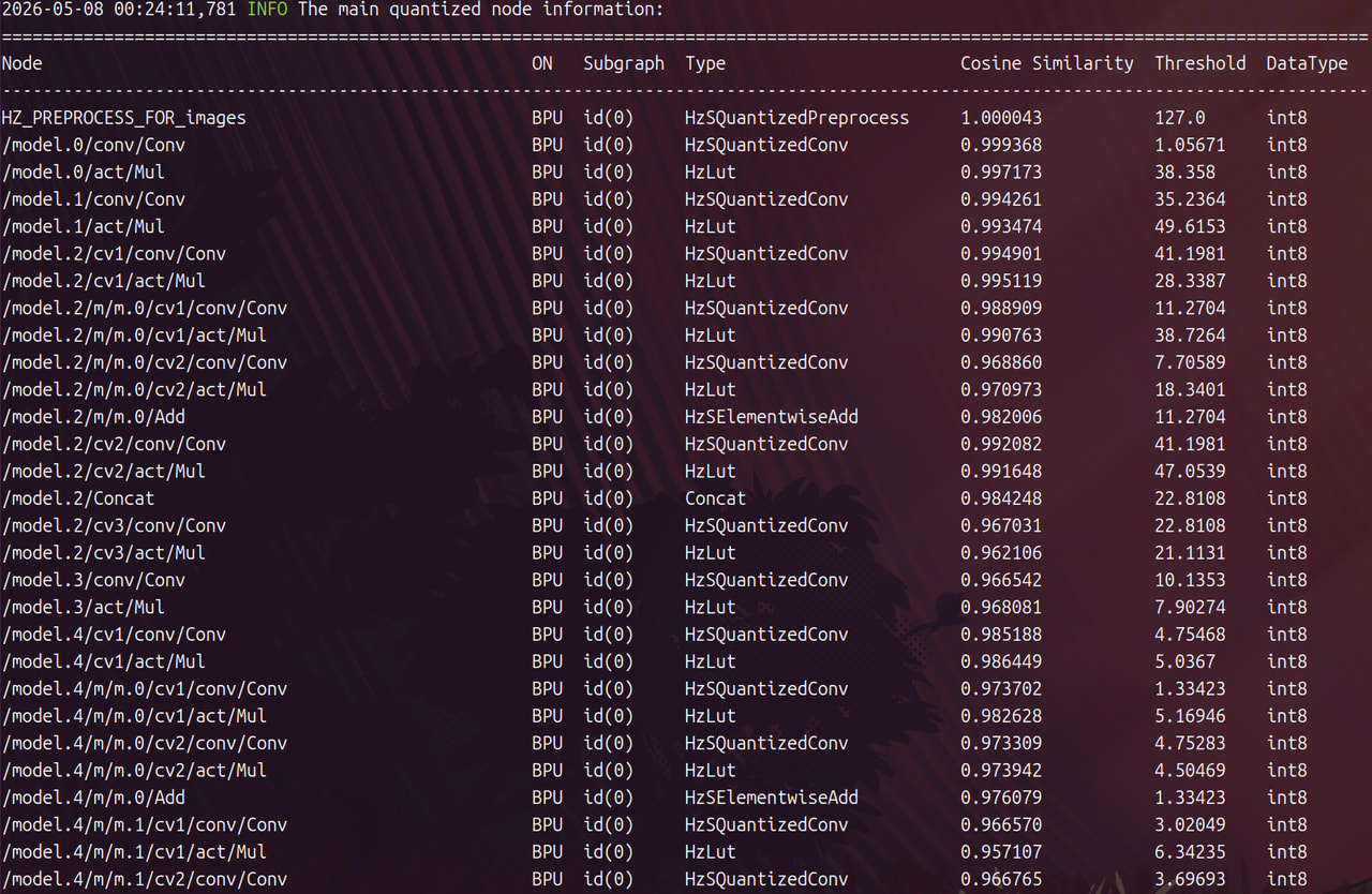
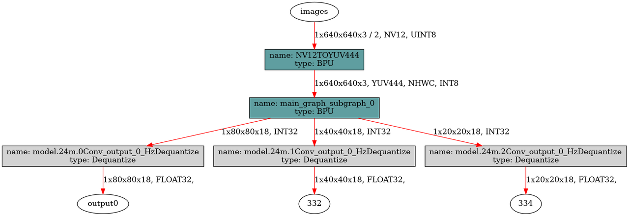
Finally, you can use hb_perf to review the quantized model architecture, as shown in the figure.
4. RDK X5 Model Deployment
4.1 Inference Pipeline on the Board
Deploy the quantized .bin model file and the inference script to the RDK X5. The core inference pipeline is: USB camera capture → NV12 preprocessing → BPU inference → post-processing → real-time display.
4.2 Inference Performance and Comparison
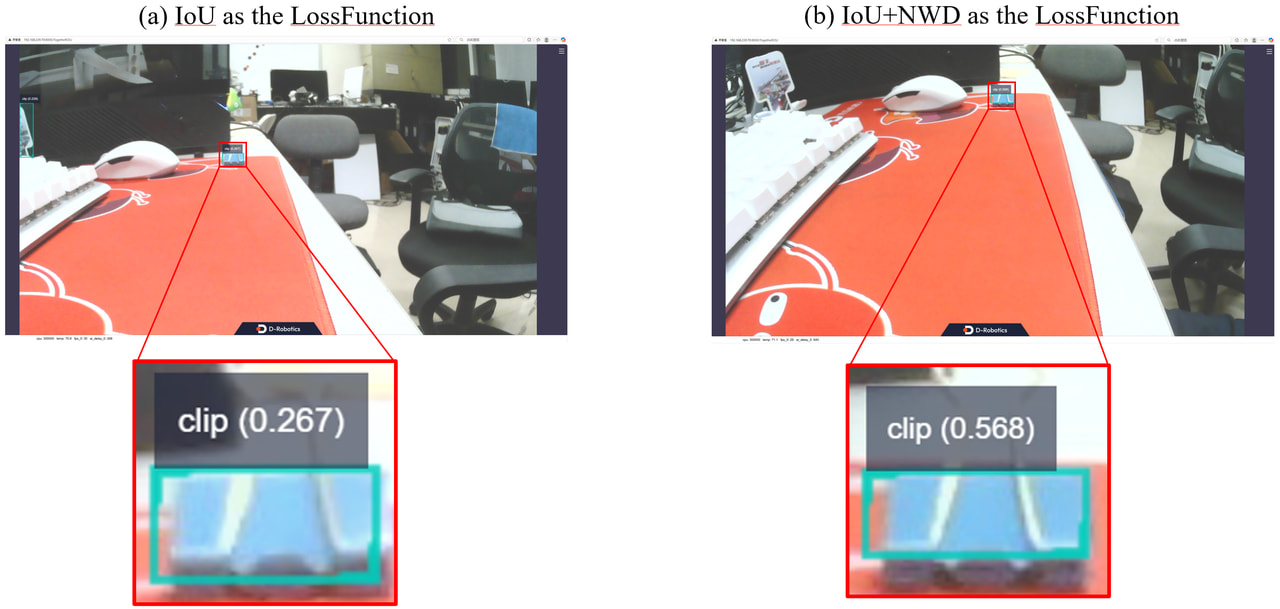
Under the same test conditions, here is a comparison between the quantized NWD-YOLOv5s and the original YOLOv5s.
| Comparison Dimension | Original YOLOv5s | NWD-YOLOv5s |
|---|---|---|
| BPU Inference FPS | Baseline | Nearly identical (loss not in inference path) |
| Confidence Score | Low, fluctuates | Significantly higher and more stable |
| Video Stream Stability | Flickering/dropped boxes | Smooth, consistent bounding boxes |
| False Positives / Misses | More frequent | Significantly reduced |
Key takeaway: The hardware acceleration during inference stays the same, while the training objective is more sensible. This brings significant improvement with no added inference latency.
4.3 Run Guide on RDK X5
Step 1. Copy the .bin model file to the RDK X5, copy config files from X5 local files.
#step 1
mkdir yolov5_nwd && cd yolov5_nwd
mkdir my_config

#step 2
## copy the .bin model file to yolov5_nwd

#step 3 copy the config files.
cp /opt/tros/humble/lib/dnn_node_example/config/yolov5workconfig.json my_config/
cp /opt/tros/humble/lib/dnn_node_example/config/coco.list my_config/
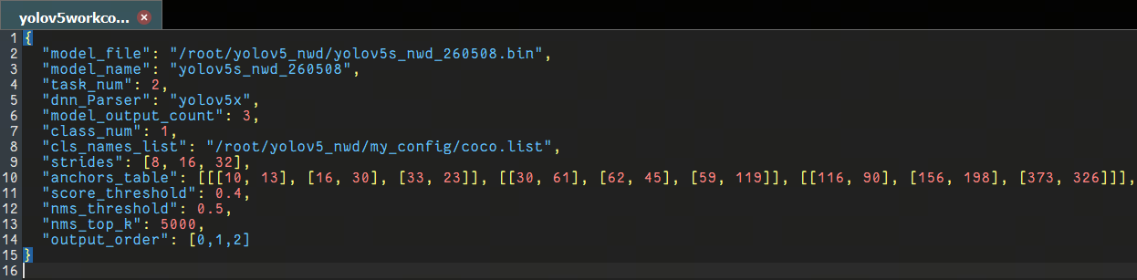
Step 2. Modify the configuration, including model path & model name, class labels & number, NMS thresholds, etc.

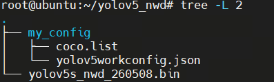
The project structure tree is shown below.
Step 3. Run the inference script and watch the real-time detection feed from the USB/mipi camera.
# Use mipi/usb camera
export CAM_TYPE=mipi #or usb

# source
source /opt/tros/humble/setup.bash
source /opt/ros/humble/setup.bash

# Run, replace your dnn_example_config_file path and camera information
ros2 launch dnn_node_example dnn_node_example.launch.py dnn_example_config_file:=my_config/yolov5workconfig.json dnn_example_image_width:=960 dnn_example_height:=544
Then, you can see the results on http://YourBoardIP:8000.
5. Future Optimization Directions (to be explored)
-
Add a small-object detection head: Introduce a higher-resolution detection layer (e.g., 160×160) in the FPN to capture fine-grained features of tiny objects.
-
Embed attention mechanisms: Add modules like CA, SE, or CBAM into the Backbone or Neck to enhance focus on small target regions.
-
Loss function weighted combination: Experiment with mixing NWD and SIoU/GIoU at different ratios to balance localization accuracy and convergence speed.
Conclusion
If you also need to detect small objects on edge devices, NWD is a low-cost optimization well worth trying. Feel free to explore more improvement directions together with the community!